Examples - Determining i or n for Known Cash Flow Values

EXAMPLE

 If Laurel made a $30,000 investment in a friend’s business and received $50,000 5 years later, determine the rate of return.

Solution 

Since only single amounts are involved,  i can be determined directly from the P/F factor.

Alternatively, the interest rate can be found by setting up the standard   P/F  relation, solving for the factor value, and interpolating in the tables.

From the interest tables, a P/F  factor of 0.6000 for  n = 5 lies between 10% and 11%. Interpolate between these two values to obtain   i = 10.76%.

EXAMPLE

Pyramid Energy requires that for each of its offshore wind power generators $5000 per year be placed into a capital reserve fund to cover unexpected major rework on field equipment. In one case, $5000 was deposited for 15 years and covered a rework costing $100,000 in year 15. What rate of return did this practice provide to the company?

Solution

The cash flow diagram is shown in  Figure 2–24 . Either the   A/F  or   F/A  factor can be used. Using A/F,

From the A /F interest tables for 15 years, the value 0.0500 lies between 3% and 4%. By interpolation,   i = 3.98%.

Figure 2–24 Diagram to determine the rate
of return

Determining i or n for Known Cash Flow Values

When all the cash flow values are known or have been estimated, the   i  value (interest rate or rate of return) or   n  value (number of years) is often the unknown. An example for which   i  is sought  may be stated as follows: A company invested money to develop a new product. After the net  annual income series is known following several years on the market, determine the rate of return  i  on the investment. There are several ways to find an unknown i or n value, depending upon the  nature of the cash flow series and the method chosen to find the unknown. The simplest case involves only single amounts (  P  and   F ) and solution utilizing a spreadsheet function. The most difficult and complex involves finding   i  or   n  for irregular cash flows mixed with uniform and  gradient series utilizing solution by hand and calculator. The solution approaches are summa-rized below, followed by examples.

Single Amounts —  P  and   F  Only 
Hand or Calculator Solution     Set up the equivalence relation and (1) solve for the variable
using the factor formula, or (2) find the factor value and interpolate in the tables. Spreadsheet Solution      Use the IRR or RATE function to find   i  or the NPER function to find n . (See below and Appendix A for details.)  

Uniform Series — A  Series
Hand or Calculator Solution      Set up the equivalence relation using the appropriate factor
(  P/A ,    A/P ,    F/A , or   A/F ), and use the second method mentioned above. Spreadsheet Solution      Use the IRR or RATE function to find   i   or the NPER function to find   n .   

Mixed A Series, Gradients, and/or Isolated Values
Hand or Calculator Solution      Set up the equivalence relation and use (1) trial and error or (2) the calculator functions. 

Spreadsheet Solution      Use the IRR or RATE function to find   i  or the NPER function to find  n . (This is the recommended approach.)

Besides the PV, FV, and NPV functions, other spreadsheet functions useful in determining   i   are IRR (internal rate of return) and RATE, and NPER (number of periods) to find   n .  The  formats  are shown here and the inside front cover with a detailed explanation in Appendix A. In all three  of these functions, at least one cash flow entry must have a sign opposite that of others in order  to find a solution.

To use IRR to find   i , enter all cash flows into contiguous cells, including zero values.

The single-cell RATE function finds   i  when an   A  series and single   P  and/or   F  values are  involved.

 NPER is a single-cell function to find  n  for single   P  and   F  values, or with an   A   series.

Engineering Economics: Introduction to Spreadsheet Use

The functions on a computer spreadsheet can greatly reduce the amount of hand work for equivalency computations involving   compound interest  and the terms   P ,  F ,  A ,  i , and   n . The use of a calculator to solve most simple problems is preferred by many students and professors as described in Appendix D. However, as cash fl  ow series become more complex, the spreadsheet offers a good alternative.  Microsoft Excel   is used throughout this book because it is readily available and easy to use. Appendix A is a primer on using spreadsheets and Excel. The functions used in engineering economy are described there in detail, with explanations of all the parameters. Appendix A also includes a section on spreadsheet layout that is useful when the economic analysis is presented to someone else—a coworker, a boss, or a professor.

A total of seven Excel functions can perform most of the fundamental engineering economy  calculations. The functions are great supplemental tools, but they do not replace the understanding of engineering economy relations, assumptions, and techniques. Using the symbols   P ,  F ,  A ,  i , and   n   defi  ned in the previous section, the functions most used in engineering economic analysis are formulated as follows.

If some of the parameters don’t apply to a particular problem, they can be omitted and zero is assumed. For readability, spaces can be inserted between parameters within parentheses. If the parameter omitted is an interior one, the comma must be entered. The last two functions require that a series of numbers be entered into contiguous spreadsheet cells, but the fi  rst fi  ve can be used  with no supporting data. In all cases, the function must be preceded by an equals sign ( = ) in the cell where the answer is to be displayed.

 To understand how the spreadsheet functions work, look back at Example 1.6  a , where the
equivalent annual amount   A  is unknown, as indicated by   A  = ?.  To  find   A  using a spreadsheet  function, simply enter the PMT function = PMT(5%,5,5000).  Figure 1–13  is a screen image  of a spreadsheet with the PMT function entered into cell B4. The answer ($1154.87) is dis- played. The answer may appear in red and in parentheses, or with a minus sign on your screen  to indicate a negative amount from the perspective of a reduction in the account balance. The  right side of  Figure 1–13  presents the solution to Example 1.6  b.  The future value   F  is determined by using the FV function. The FV function appears in the formula bar; and many examples throughout this text will include cell tags, as shown here, to indicate the format of  important entries.

The following example demonstrates the use of a spreadsheet to develop relations (not built-in functions) to calculate interest and cash fl ows. Once set up, the spreadsheet can be used to perform sensitivity analysis for estimates that are subject to change. We will illustrate the use of spreadsheets throughout the chapters. (  Note:  The spreadsheet examples may be omitted, if spreadsheets are not used in the course. A solution by hand is included in virtually all examples.)

EXAMPLE 1.6

  Figure 1–13  Use of spreadsheet functions PMT and FV, Example 1.6.

EXAMPLE 1.17

A Japan-based architectural fi rm has asked a United States–based software engineering group to infuse GPS sensing capability via satellite into monitoring software for high-rise structures in order to detect greater than expected horizontal movements. This software could be very beneficial as an advance warning of serious tremors in earthquake-prone areas in Japan and the United States. The inclusion of accurate GPS data is estimated to increase annual revenue over that for the current software system by $200,000 for each of the next 2 years, and by $300,000 for each of years 3 and 4. The planning horizon is only 4 years due to the rapid advances made internationally in building-monitoring software. Develop spreadsheets to answer the questions below.  

  (a)    Determine the total interest and total revenue after 4 years, using a compound rate of return of 8% per year. 
  (b)    Repeat  part  (  a ) if estimated revenue increases from $300,000 to $600,000 in years 3 and 4.  
  (c)    Repeat  part  (  a ) if infl ation is estimated to be 4% per year. This will decrease the   real rate  of return  from 8% to 3.85% per year (Chapter 14 shows why).

Solution by Spreadsheet

Refer to  Figure 1–14   a  to   d  for the solutions. All the spreadsheets contain the same information,  but some cell values are altered as required by the question. (Actually, all the questions can be  answered on one spreadsheet by changing the numbers. Separate spreadsheets are shown here  for explanation purposes only.)

The Excel functions are constructed with reference to the cells, not the values them- selves, so that sensitivity analysis can be performed without function changes. This ap- proach treats the value in a cell as a   global variable  for the spreadsheet. For example, the  8% rate in cell B2 will be referenced in all functions as B2, not 8%. Thus, a change in the  rate requires only one alteration in the cell B2 entry, not in every relation where 8% is used.  See Appendix A for additional information about using cell referencing and building  spreadsheet relations. 

(a)   Figure  1–14  a  shows the results, and  Figure 1–14  b  presents all spreadsheet relations for  estimated interest and revenue (yearly in columns C and E, cumulative in columns D  and F). As an illustration, for year 3 the interest   I3  and revenue plus interest   R3   are

The equivalent amount after 4 years is $1,109,022, which is comprised of $1,000,000 in  total revenue and $109,022 in interest compounded at 8% per year. The shaded cells in  Figure  1–14  a  and   b  indicate that the sum of the annual values and the last entry in the cu- mulative columns must be equal.  

(b)  To determine the effect of increasing estimated revenue for years 3 and 4 to $600,000,  use the same spreadsheet and change the entries in cells B8 and B9 as shown in Figure  1–14  c . Total interest increases 22%, or $24,000, from $109,222 to $133,222.

(c)   Figure  1–14  d  shows the effect of changing the original   i  value from 8% to an infl  ation- adjusted rate of 3.85% in cell B2 on the fi rst spreadsheet. [Remember to return to the  $300,000 revenue estimates for years 3 and 4 after working part (  b ).]  Infl  ation has now reduced total interest by 53% from $109,222 to $51,247, as shown in cell C10.

 Figure 1–14   Spreadsheet solutions with sensitivity analysis, Example 1.17  a  to   c .

Comment

Later we will learn how to utilize the NPV and FV Excel fi nancial functions to obtain the same  answers determined in  Figure 1–14 , where we developed each basic relation.  When you are working with an Excel spreadsheet, it is possible to display all of the entries  and functions on the screen as shown in  Figure 1–14   b  by simultaneously touching the <Ctrl> and < `> keys, which may be in the upper left of the keyboard on the key with <~>.

Economic Equivalence

Economic equivalence is a fundamental concept upon which engineering economy computations are based. Before we delve into the economic aspects, think of the many types of equivalency we may utilize daily by transferring from one scale to another. Some example transfers between scales are as follows:

Often equivalency involves two or more scales. Consider the equivalency of a   speed  of 110 kilometers per hour (kph) into miles per minute using conversions between distance and time scales with three-decimal accuracy.

Four scales—time in minutes, time in hours, length in miles, and length in kilometers—are combined to develop these equivalent statements on speed. Note that throughout these statements, the fundamental relations of 1 mile = 1.609 kilometers and 1 hour = 60 minutes are applied. If a fundamental relation changes, the entire equivalency is in error.

Now  we  consider  economic  equivalency.         

Economic equivalence  is a combination of   interest rate and  time value of money  to determine the different amounts of money at different points in time that are equal in economic value. 

As an illustration, if the interest rate is 6% per year, $100 today (present time) is equivalent to $106 one year from today.

  Amount  accrued = 100 + 100(0.06) = 100(1 + 0.06) = $106

If someone offered you a gift of $100 today or $106 one year from today, it would make no difference which offer you accepted from an economic perspective. In either case you have $106 one year from today. However, the two sums of money are equivalent to each other   only  when the interest rate is 6% per year. At a higher or lower interest rate, $100 today is not equivalent to $106  one year from today.

In addition to future equivalence, we can apply the same logic to determine equivalence for previous years. A total of $100 now is equivalent to $100 1.06 = $94.34 one year ago at an interest rate of 6% per year. From these illustrations, we can state the following: $94.34 last year, $100 now, and $106 one year from now are equivalent at an interest rate of 6% per year. The fact that these sums are equivalent can be verifi ed by computing the two interest rates for 1-year interest periods.

The cash flow diagram in  Figure 1–10  indicates the amount of interest needed each year to make these three different amounts equivalent at 6% per year.

  Figure 1–10  Equivalence of money at 6% per year interest.

EXAMPLE 1.12

Manufacturers make backup batteries for computer systems available to Batteries + dealers through privately owned distributorships. In general, batteries are stored throughout the year,  and a 5% cost increase is added each year to cover the inventory carrying charge for the distributorship owner. Assume you own the City Center Batteries  + outlet. Make the calculations necessary to show which of the following statements are true and which are false about battery costs.

(a)    The amount of $98 now is equivalent to a cost of $105.60 one year from now.
(b)    A truck battery cost of $200 one year ago is equivalent to $205 now.
(c)    A $38 cost now is equivalent to $39.90 one year from now.
(d)    A $3000 cost now is equivalent to $2887.14 one year earlier.
(e)    The carrying charge accumulated in 1 year on an investment of $20,000 worth of  batteries is $1000.

Comparison of alternative cash flow series requires the use of equivalence to determine when the series are economically equal or if one is economically preferable to another. The keys to the analysis are the interest rate and the timing of the cash flows. Example 1.13 demonstrates how easy it is to be misled by the size and timing of cash flows.

EXAMPLE 1.13

Howard owns a small electronics repair shop. He wants to borrow $10,000 now and repay it over the next 1 or 2 years. He believes that new diagnostic test equipment will allow him to work on a wider variety of electronic items and increase his annual revenue. Howard received 2-year repayment options from banks A and B.

After reviewing these plans, Howard decided that he wants to repay the $10,000 after only 1 year based on the expected increased revenue. During a family conversation, Howard’s brother-in-law offered to lend him the $10,000 now and take $10,600 after exactly 1 year. Now Howard has three options and wonders which one to take. Which one is economically the best?

Solution

The repayment plans for both banks are economically equivalent at the interest rate of 5% per year. (This is determined by using computations that you will learn in Chapter 2.) Therefore,  Howard can choose either plan even though the bank B plan requires a slightly larger sum of  money over the 2 years.

The brother-in-law repayment plan requires a total of $600 in interest 1 year later plus the  principal of $10,000, which makes the interest rate 6% per year. Given the two 5% per year  options from the banks, this 6% plan should not be chosen as it is not economically better than  the other two. Even though the sum of money repaid is smaller, the timing of the cash flows  and the interest rate make it less desirable.   The point here is that cash flows themselves, or  their sums, cannot be relied upon as the primary basis for an economic decision. The interest  rate, timing, and economic equivalence must be considered. 

Interest Rate and Rate of Return

Interest  is the manifestation of the time value of money. Computationally, interest is the difference between an ending amount of money and the beginning amount. If the difference is zero or negative, there is no interest. There are always two perspectives to an amount of interest—interest paid and interest earned. These are illustrated in  Figure 1–2 . Interest is   paid  when a person or organization borrowed money (obtained a loan) and repays a larger amount over time. Interest is  earned  when a person or organization saved, invested, or lent money and obtains a return of a larger amount over time. The numerical values and formulas used are the same for both perspectives, but  the interpretations are different.  

Interest paid  on borrowed funds (a loan) is determined using the original amount, also called the principal,

  Interest = amount owed now - principal                            [1.1]

When interest paid over a   specific time unit  is expressed as a percentage of the principal, the result is called the interest rate.

The time unit of the rate is called the   interest period.  By far the most common interest period used to state an interest rate is 1 year. Shorter time periods can be used, such as 1% per month. Thus, the interest period of the interest rate should always be included. If only the rate is stated, for example, 8.5%, a 1-year interest period is assumed.

  Figure 1–2   (a) Interest paid over time to lender. (b) Interest earned over time by investor.

From the perspective of a saver, a lender, or an investor,  interest earned  ( Figure  1–2  b ) is the  final amount minus the initial amount, or principal.

  Interest  earned total amount now principal           [1.3]

Interest earned over a specific period of time is expressed as a percentage of the original amount and is called rate of return (ROR).

 The time unit for rate of return is called the interest period,  just as for the borrower’s perspec-
tive. Again, the most common period is 1 year.

The term  return on investment (ROI)  is used equivalently with ROR in different industries and  settings, especially where large capital funds are committed to engineering-oriented  programs.  

The numerical values in Equations [1.2] and [1.4] are the same, but the term   interest rate paid
is more appropriate for the borrower’s perspective, while the   rate of return earned  is better for
the investor’s perspective.

In Examples 1.3 to 1.5 the interest period was 1 year, and the interest amount was calculated  at the end of one period. When more than one interest period is involved, e.g., the amount of interest after 3 years, it is necessary to state whether the interest is accrued on a simple or compound  basis from one period to the next. This topic is covered later in this chapter.

Since   inflation   can  significantly increase an interest rate, some comments about the funda- mentals of inflation are warranted at this early stage. By definition, inflation represents a decrease  in the value of a given currency. That is, $10 now will not purchase the same amount of gasoline  for your car (or most other things) as $10 did 10 years ago. The changing value of the currency affects market interest rates.

In simple terms, interest rates reflect two things: a so-called real rate of return   plus  the  expected  inflation rate. The real rate of return allows the investor to purchase more than he or she could  have purchased before the investment, while inflation raises the real rate to the market rate that  we use on a daily basis.

The safest investments (such as government bonds) typically have a 3% to 4% real rate of  return built into their overall interest rates. Thus, a market interest rate of, say, 8% per year on a  bond means that investors expect the inflation rate to be in the range of 4% to 5% per year.  Clearly, inflation causes interest rates to rise.

From the borrower’s perspective, the rate of inflation is another interest rate   tacked on to the  real interest rate . And from the vantage point of the saver or investor in a fixed-interest account, inflation   reduces the real rate of return  on the investment. Inflation means that cost and revenue  cash flow estimates increase over time. This increase is due to the changing value of money that  is forced upon a country’s currency by inflation, thus making a unit of currency (such as the dollar) worth less relative to its value at a previous time. We see the effect of inflation in that money  purchases less now than it did at a previous time. Inflation contributes to

   •     A reduction in purchasing power of the currency
   •     An increase in the CPI (consumer price index)
   •     An increase in the cost of equipment and its maintenance
   •     An increase in the cost of salaried professionals and hourly employees
   •     A reduction in the real rate of return on personal savings and certain corporate investments

In other words, inflation can materially contribute to changes in corporate and personal economic  analysis.
  
Commonly, engineering economy studies assume that inflation affects all estimated values  equally. Accordingly, an interest rate or rate of return, such as 8% per year, is applied throughout  the analysis without accounting for an additional inflation rate. However, if inflation were explicitly taken into account, and it was reducing the value of money at, say, an average of 4% per year,  then it would be necessary to perform the economic analysis using an inflated interest rate.

EXAMPLE 1.3

An employee at LaserKinetics.com borrows $10,000 on May 1 and must repay a total of  $10,700 exactly 1 year later. Determine the interest amount and the interest rate paid.

Solution

The perspective here is that of the borrower since $10,700 repays a loan. Apply Equation [1.1]  to determine the interest paid.

EXAMPLE 1.4

Stereophonics, Inc., plans to borrow $20,000 from a bank for 1 year at 9% interest for new recording equipment. (  a ) Compute the interest and the total amount due after 1 year. (  b )  Construct a column graph that shows the original loan amount and total amount due after 1 year used to compute the loan interest rate of 9% per year.

Solution

  Figure 1–3  Values used to compute an interest rate of 9% per year. Example 1.4.

Comment

Note that in part (  a ), the total amount due may also be computed as

     Total  due = principal(1 + interest rate) = $20,000(1.09) = $21,800

Later we will use this method to determine future amounts for times longer than one interest period.

EXAMPLE 1.5

(a)    Calculate the amount deposited 1 year ago to have $1000 now at an interest rate of 5%  per year.  (b)    Calculate the amount of interest earned during this time period.  

Solution

Compute the Future Value, Knowing the Following Cash Flow.

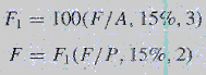
Using a 15% interest rate, compute the value of F in the following cash flow:

SOLUTION

Looked at this way, we first solve for Fl.

Now F1 can be considered a present sum P in the diagram

The slightly different value from the preceding computation is due to rounding in the compound interest tables.

This has been a two-step solution:

One could substitute the value of F1 from the first equation into the second equation and solve for F, without computing Fl,

UNIFORM SERIES COMPOUND INTEREST FORMULAS.

Many times we will find uniform series of receipts or disbursements. Automobile loans, house payments, and many other loans are based on a uniform payment series. It will often be convenient to use tables based on a uniform series of receipts or disbursements.

The series A is definedas follows:


A = An end-of-periodl cash receipt or disbursementin a uniform series, continuing for n periods, the entire series equivalent to P or F at interest rate i

The horizontal line in Figure 4-1 is a representation of time with four interest periods illustrated. Uniform payments A have been placed at the end of each interest period, and there are as many A's as there are interest periods n. (Both these conditions are specifiedin the definitionof A.) Figure 4-1 uses January 1 and December 31, but other 1-year periods could be used.

We will use this relationship in our uniform series derivation.

Figure 4-1  The general relationship between A and F.

1 In textbooks on economic analysis, it is customary to define A as an end-of-period event rather than a.
beginning-of-period or, possibly, middle-of-period event. The derivations that follow are based on this
end-of-period assumption. One could, of course, derive other equations based on beginning-of-period
or mid period assumptions.

Looking at Figure 4-1,we see that if an amount A is investedat the end of each year for 4 years, the total amount F at the end of 4 years will be the sum of the compound amounts of the individual investments.

In the general case for n years,

Multiplying Equation (4-1) by (1 + i), we have .

Factoring out A and subtracting Equation 4-1 gives

Solving Equation 4-4 for F gives

Thus we have an equation for F when A is known. The term inside the brackets 

is called the uniformseries compound amount factor and has the notation (F/A, i,n).

Example: Equivalence Calculations - Solve P.

Consider the following situation:

Solve for P assuming a 12% interest rate and using the compound interest tables. Recall that receipts have a plus sign and disbursements or payments have a negative sign. Thus, the diagram is:

SOLUTION

It its important to understandjust what the solution, $625.16, represents.We can say that $625.16
is tbe amount of moneythat would need to be invested at 12% annual interest to allow for the withdrawal of $400 at the end of 3 years and $600 at the end of 5 years.

Let's examine the computations further.
If  $625.16 is invested for one year at 12% interest, it will increase to [625.16+0.12(625.16)] = $700.18. If for the second year the $700.18 is invested at 12%, it will increase to [700.18+0.12(700.18)] = $784.20. And if this is repeated for another year, [784.20+ 0.12(784.20)] =$878.30.

We are now at the end of Year 3. The original $625.16 has increased through the addition of interest to $878.30. It is at this point that the $400 is paid out. Deducting $400 from $878.30 leaves $478.30.

The $478.30 can be invested at 12%for the fourth year and will increase to [478.30+0.12(478.30)] =$535.70.Andifleft at interest for anotheryear, itwill increaseto [535.70+0.12(535.70)] = $600.We are now at the end of Year 5; with a $600 payout; there is money remaining in the account.

In other words, the $625.16 was just enough money,at a 12%interest rate, to exactly provide for a $400 disbursement at the end of Year 3 and also a $60 0disbursement at the end of Year 5. Weend up neither short of moneyn or with money left over: this is an illustration of equivalence.The initial $625.16 is equivalent to the combination of a $400 disbursement at the end of Year 3 and a $600 disbursementat the end of Year 5.

Example: Equivalence Calculations - Time Valued of Money.

If  $500 were deposited in a bank savings account,how muchwould be in the account three years hence if the bank paid 6% interest compounrted anually?

We can draw a diagramof the problem. [Note:To have a consistent notation, we will represent receipts by upward arrows (and positive signs), and disbursements (or payments) will have downward arrows (and negative signs).]

SOLUTION

From the view point of the person depositing the $500, the diagram for "today" (Time=0) through
Year 3 is as follows:

Weneed to identify the various elementsof the equation.The present sum P is $500.The interest rate per interest period is 6%, and in 3 years there are three interest periods. The future sum F is to be computed from the formula

SINGLE PAYMENT COMPOUND INTEREST FORMULAS - TIME VALUE OF MONEY.

To facilitate equivalence computations, a series of interest formulas will be derived. To simplify the presentation, we'll use the following notation:

Suppose a present sum of money P is invested for one year l at interest rate i. At the end of the year, we should receive back our initial investment P, together with interest equal to iP, or a total amount P + iP. Factoring P, the sum at the end of one year is P(1 + i).

Let us assume that, instead of removing our investment at the end of one year, we agree to let it remain for another year. How much would our investment be worth at the end of the second year? The end-of-first-year sum P(1 + i) will draw interest in the second year of. i P(1 + i). Thismeans that, at the end of the second year, the total investmentwill become

1 A more general statement is to specify "one interest period" rather than "one year." Since, however,
it is easier to visualize one year, the derivation will assume that one year is the interest period.

This may be rearranged by factoring P(1 + i), which gives us

In other words, a present sum P increases in n periods to P(1 + i)^n. We therefore have a relationship between a present sum P and its equivalentfuture sum, F.

This is the single payment compound amount formula and is written in functional notation as

The notation in parentheses (F/P, i, n) can be read as follows:

To find a future sum F, given a present sum, P, at an interest rate i per interest period,
and n interest periods hence. .

Functional notation is designed so that the compound interest factors may be written in an equation in an algebraically correct form. In Equation 3-4, for example, the functional mnotation is interpreted as

which is dimensionally correct.Without proceeding further, we can see that when we derive. a compound interest factor to find a present sum P, given a future sum F, the factor will
be (P/F, i, n); so, the resulting equation would be

which is dimensionally correct.